Usage

Basic example

Import AISim plus numpy and matplotlib and print current version:

import numpy as np
import matplotlib.pyplot as plt
import aisim as ais
from functools import partial
print(ais.__version__)

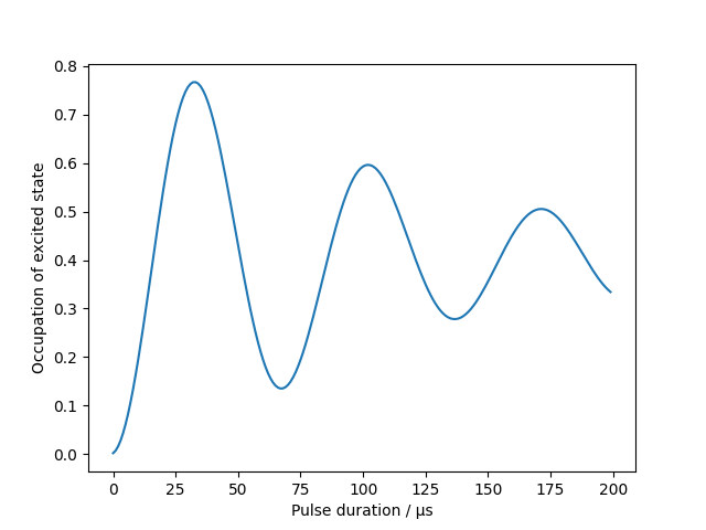
As an example, we simulate Rabi oscillations driven by stimulated Raman transitions in the presence of thermal motion.

Note

If not explicitly stated otherwise in the docstring, units are assumed to be SI units without prefixes, i.e. meters or Kelvin. The only exception is kilogram.

First, we define a AtomicEnsemble object for atoms from a magneto-optical trap after sub-Doppler cooling:

# Generate an AtomicEnsemble of 10000 atoms in the ground state, in aspherical
# atomic cloud with radius 3 mm with velocity spread in m/s at temperature of 3 μK
# in x and y, and 150 nK in z (after a velocity selection process):
atoms = ais.create_random_ensemble(
int(1e4),
x_dist=partial(ais.dist.position_dist_gaussian, std=3.0e-3),
y_dist=partial(ais.dist.position_dist_gaussian, std=3.0e-3),
z_dist=partial(ais.dist.position_dist_gaussian, std=3.0e-3),
vx_dist=partial(ais.dist.velocity_dist_from_temp, temperature=3.0e-6),
vy_dist=partial(ais.dist.velocity_dist_from_temp, temperature=3.0e-6),
vz_dist=partial(ais.dist.velocity_dist_from_temp, temperature=150e-9),
seed=1,

)

Only a fraction of these atoms will be detected after a time-of-flight of 800 ms. We model the detection region with radius of 5 mm:

det = ais.SphericalDetector(t_det=800e-3, r_det=5e-3)

We select the atoms that are eventually detected, let those freely propagate for 100 ms

We setup the two counter-propagating Raman laser beams with a wavelength of 780 nm, 30 mm beam diameter and a Rabi frequency of 15 kHz as IntensityProfile and WaveVectors objects:

We select the atoms that are eventually detected, let those freely propagate for 100 ms before we start the Rabi oscillations up to 200 μs:

atoms = det.detected_atoms(atoms)
atoms = ais.prop.free_evolution(atoms, dt=100e-3)

state_occupation = []
taus = np.arange(200) * time_delta
for tau in taus:
    atoms = prop.propagate(atoms)
    mean_occupation = np.mean(atoms.state_occupation(state=1))
    state_occupation.append(mean_occupation)

Finally, we plot the results:

fig, ax = plt.subplots()
ax.plot(1e6 * taus, state_occupation)
ax.set_xlabel("Pulse duration / μs")
ax.set_ylabel("Occupation of excited state");

More examples

The notebooks containing the following exampels can also be found here: